12. Differentials & Linear Approximation
b. Linear Approximation
Given a function \(y=f(x)\), pick a fixed point \(x=a\) and nearby variable point \(x\). If \(x\) is close to \(a\), then \(f_{\tan}(x)\) is close to \(f(x)\). Further, since \[ df=f_{\tan}(x)-f(a) \] and \[ \Delta f=f(x)-f(a), \] we have \(df\) is also close to \(\Delta f\).
Notice in the animation that as \(x\) approaches \(a\), \(f(x)\) seems to merge with \(f_{\tan}(x)\) before they both approach \(f(a)\). Further, \(\Delta f\) gets close to \(df\).
\(y=f(x)\) near \(x=a\).
If \(x\) is close to \(a\), then \(f_{\tan}(x)\) is a good approximation to \(f(x)\) and \(df\) is a good approximation to \(\Delta f\). In symbols: \[ f(x) \approx f_{\tan}(x) \qquad \qquad \Delta f \approx df \]
Problems on applications of linear approximations can either be simple and of limited use or moderate difficulty and practical. The former category generally encompasses problems requiring you to estimate the value of an expression:
Estimating the value of an expression
Use a linear approximation to estimate \(\sqrt{4.1}\).
Note: We
previously found the derivative of \(f(x)=\sqrt{x}\) is
\(f'(x)=\dfrac{1}{2\sqrt{x}}\). It can also be found using the
Power Rule, \(\dfrac{d}{dx}x^n=nx^{n-1}\), with \(n=\dfrac{1}{2}\)
even though \(n\) is not a positive integrer. Specifically:
\[
\dfrac{d}{dx}\sqrt{x}=\dfrac{d}{dx}x^{1/2}=\dfrac{1}{2}x^{-1/2}=\dfrac{1}{2\sqrt{x}}
\]
We take \(f(x)=\sqrt{x}\), since we know \(f(4)=2\). We then construct the tangent function. We have: \[ f'(x)=\dfrac{1}{2\sqrt{x}} \qquad \qquad f'(4)=\dfrac{1}{2\sqrt{4}}=\dfrac{1}{4} \] So: \[f_{\tan}(x)=f(4)+f'(4)(x-4)=2+\dfrac{1}{4}(x-4)\] (Note: We don't simplify because the next step is easier without simplification.) Finally, let \(x=4.1\). Then \[ \sqrt{4.1}=f(4.1)\approx f_{\tan}(4.1) =2+\dfrac{1}{4}(4.1-4)=2+\dfrac{.1}{4}=2.025 \] (Note: Using a calculator, the actual value is \(\sqrt{4.1}=2.0248456\). So this is a good approximation.)
Problems like this are "dumb" because it is easier to just plug it into your calculator and get a better value. However, this is basically what a calculator or computer does when it numerically estimates a value. It uses a linear approximation (or higher degree Taylor approximation) to reach the desired degree of accuracy.
Use a linear approximation to estimate \(\dfrac{1}{\sqrt{15.8}}\).
Note: We
previously found the derivative of \(f(x)=\dfrac{1}{\sqrt{x}}\) is
\(f'(x)==\dfrac{-1}{2x^{3/2}}\). Alternatively, we can use the
Power Rule formula, \(\dfrac{d}{dx}x^n=nx^{n-1}\), with \(n=-\,\dfrac{1}{2}\)
even though \(n\) is not a positive integrer. Specifically:
\[
\dfrac{d}{dx}\dfrac{1}{\sqrt{x}}=\dfrac{d}{dx}x^{-1/2}
=-\,\dfrac{1}{2}x^{-3/2}=\dfrac{-1}{2x^{3/2}}
\]
\(\dfrac{1}{\sqrt{15.8}}\approx.2515625\)
We take \(f(x)=\dfrac{1}{\sqrt{x}}\) since we know \(f(16)=\dfrac{1}{4}\). We then construct the tangent function. We have: \[ f'(x)=\dfrac{-1}{2x^{3/2}} \qquad f'(16)=\dfrac{-1}{2\cdot16^{3/2}} =\dfrac{-1}{128} \] So: \[\begin{aligned} f_{\tan}(x) &=f(16)+f'(16)(x-16) \\ &=\dfrac{1}{4}-\dfrac{1}{128}(x-16) \end{aligned}\] Finally, we let \(x=15.8\). Then \[\begin{aligned} \dfrac{1}{\sqrt{15.8}} &=f(15.8) \approx f_{\tan}(15.8) \\ &=\dfrac{1}{4}-\dfrac{1}{128}(15.8-16) \\ &=.25+\dfrac{.2}{128}=.2515625 \end{aligned}\] (Note: Using a calculator, the actual value is \(\dfrac{1}{\sqrt{15.8}}=.251577\). So this is a really good approximation.)
More reasonable problems occur in applications.
Applications of LinearApproximations
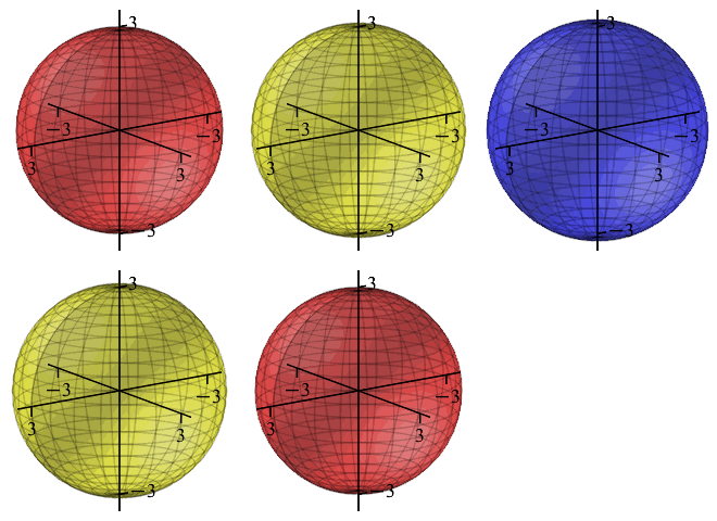
If the radius of a sphere is measured to be \(r=3\,\text{cm}\pm.02\,\text{cm}\),
find the volume of the sphere and estimate the error in this
computed value of the volume. (Give answers as multiples of \(\pi\).)
red: \(r=2.98\)
yellow: \(\ \ r=3\)
blue: \(\quad r=3.02\)

The volume is \[ V=\dfrac{4}{3}\pi r^3=\dfrac{4}{3}\pi3^3=36\pi \] The error in the measurement of the radius can be regarded as a change in the radius: \[\Delta r=.02\] Then the error in the volume is the corresponding change in the volume which may be approximated by the differential: \[ \Delta V\approx dV=\dfrac{dV}{dr}\,dr =4\pi r^2\,dr=4\pi3^2\cdot.02=.72\pi \] So we say \(V=36\pi\,\text{cm}^3\pm.72\pi\,\text{cm}^3\).
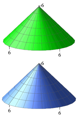
A bucket of sand is hanging from a tree and leaking to form a conical pile whose height is always equal to its radius. At present, the radius (and height) is \(r=h=6\,\text{cm}\) (shown in green) and so the volume is \[ V=\dfrac{1}{3}\pi r^2 h=\dfrac{1}{3}\pi r^3 =\dfrac{1}{3}\pi6^3=72\pi\,\text{cm}^3 \] If the volume is increased by \(6\pi\,\text{cm}^3\) (shown in blue), use the linear approximation to estimate the the increase in radius (and height).

\(\Delta r=\Delta h\approx\dfrac{1}{6}\)
The change in volume is \(\Delta V=6\pi\) and we want to estimate the change in radius \(\Delta r\). The linear approximation says these are approximated by the differential of volume \(dV\) and the differential of radius \(dr\). Since the volume is \(V=\dfrac{1}{3}\pi r^3\), the differentials are related by \[ dV=\dfrac{dV}{dr}\,dr=\pi r^2\,dr \] We solve for \(dr\) and plug in numbers: \[ \Delta r\approx dr=\dfrac{dV}{\pi r^2}=\dfrac{6\pi}{\pi 6^2}=\dfrac{1}{6} \]
Boyle's Law says that for an ideal gas at constant Temperature, the Pressure is inversely proportional to the Volume. Suppose the Volume and Pressure are initially \(V_i=30\,\text{cm}^3\) and \(P_i=1.2\,\text{atm}\). If the volume is increased by \(\Delta V=0.2\,\text{cm}^3\), use the linear approximation to estimate the change in the pressure \(\Delta P\) and the final pressure \(P_f\).
\(\Delta P\approx-.008\)
\(P_f=1.192\)
Boyle's Law says \(P=\dfrac{K}{V}\). We use the initial values of \(P\) and \(V\) to find \[ K=PV=(1.2)(30)=36 \] The change in pressure is estimated by its differential \[ \Delta P\approx dP=\dfrac{dP}{dV}\,dV=\dfrac{-K}{V^2}\,dV =\dfrac{-36}{30^2}0.2=-.008 \] So the final pressure is \[ P_f=P_i+\Delta P\approx1.2-.008=1.192 \]
Heading
Placeholder text: Lorem ipsum Lorem ipsum Lorem ipsum Lorem ipsum Lorem ipsum Lorem ipsum Lorem ipsum Lorem ipsum Lorem ipsum Lorem ipsum Lorem ipsum Lorem ipsum Lorem ipsum Lorem ipsum Lorem ipsum Lorem ipsum Lorem ipsum Lorem ipsum Lorem ipsum Lorem ipsum Lorem ipsum Lorem ipsum Lorem ipsum Lorem ipsum Lorem ipsum